Example 10: Analyzing the Results of the High-Lat Run

In this Example we analyze the results of an MPI run of NPTFit performed over high latitudes.

The example batch script we provide, Example10_HighLat_Batch.batch is for SLURM. This calls the run file Example10_HighLat_Run.py using MPI, and is an example of how to perform a more realistic analysis using NPTFit.

NB: The batch file must be run before this notebook.

NB: This example makes use of the Fermi Data, which needs to already be installed. See Example 1 for details.

In this example, we model the source-count function as a triply-broken power law. In detail, the source count function is then:

\[\begin{split}\frac{dN}{dS} = A \left\{ \begin{array}{lc} \left( \frac{S}{S_{b,1}} \right)^{-n_1}, & S \geq S_{b,1} \\ \left(\frac{S}{S_{b,1}}\right)^{-n_2}, & S_{b,1} > S \geq S_{b,2} \\ \left( \frac{S_{b,2}}{S_{b,1}} \right)^{-n_2} \left(\frac{S}{S_{b,2}}\right)^{-n_3}, & S_{b,2} > S \geq S_{b,3} \\ \left( \frac{S_{b,2}}{S_{b,1}} \right)^{-n_2} \left( \frac{S_{b,3}}{S_{b,2}} \right)^{-n_3} \left(\frac{S}{S_{b,3}}\right)^{-n_4}, & S_{b,3} > S \end{array} \right.\end{split}\]

and is thereby described by the following eight parameters:

\[\theta = \left[ A, n_1, n_2, n_3, n_4, S_b^{(1)}, S_b^{(2)}, S_b^{(3)} \right]\,.\]

This provides an example of a more complicated source count function, and also explains why the run needs MPI.

# Import relevant modules

%matplotlib inline
%load_ext autoreload
%autoreload 2

import numpy as np
import corner
import matplotlib.pyplot as plt

from NPTFit import nptfit # module for performing scan
from NPTFit import create_mask as cm # module for creating the mask
from NPTFit import dnds_analysis # module for analysing the output
from NPTFit import psf_correction as pc # module for determining the PSF correction

from __future__ import print_function

Load in scan

We need to create an instance of nptfit.NPTF and load in the scan performed using MPI.

n = nptfit.NPTF(tag='HighLat_Example')

fermi_data = np.load('fermi_data/fermidata_counts.npy').astype(np.int32)
fermi_exposure = np.load('fermi_data/fermidata_exposure.npy')
n.load_data(fermi_data, fermi_exposure)

analysis_mask = cm.make_mask_total(band_mask = True, band_mask_range = 50)
n.load_mask(analysis_mask)

dif = np.load('fermi_data/template_dif.npy')
iso = np.load('fermi_data/template_iso.npy')

n.add_template(dif, 'dif')
n.add_template(iso, 'iso')
n.add_template(np.ones(len(iso)), 'iso_np', units='PS')

n.add_poiss_model('dif','$A_\mathrm{dif}$', [0,20], False)
n.add_poiss_model('iso','$A_\mathrm{iso}$', [0,5], False)

n.add_non_poiss_model('iso_np',
                      ['$A^\mathrm{ps}_\mathrm{iso}$',
                      '$n_1$','$n_2$','$n_3$','$n_4$',
                      '$S_b^{(1)}$','$S_b^{(2)}$','$S_b^{(3)}$'],
                      [[-6,2],
                      [2.05,5],[1.0,3.5],[1.0,3.5],[-1.99,1.99],
                      [30,80],[1,30],[0.1,1]],
                      [True,False,False,False,False,False,False,False])

pc_inst = pc.PSFCorrection(psf_sigma_deg=0.1812)
f_ary, df_rho_div_f_ary = pc_inst.f_ary, pc_inst.df_rho_div_f_ary

Loading the psf correction from: /zfs/nrodd/NPTFRemakeExamples/psf_dir/gauss_128_0.181_10_50000_1000_0.01.npy

n.configure_for_scan(f_ary=f_ary, df_rho_div_f_ary=df_rho_div_f_ary, nexp=5)

The number of parameters to be fit is 10

Finally, load the completed scan performed using MPI.

n.load_scan()

analysing data from /zfs/nrodd/NPTFRemakeExamples/chains/HighLat_Example/.txt

Analysis

As in Example 9 we first initialize the analysis module. We will provide the same basic plots as in that notebook, where more details on each option is provided.

an = dnds_analysis.Analysis(n)

1. Make triangle plots

an.make_triangle()

2. Get Intensities

print("Iso NPT Intensity",corner.quantile(an.return_intensity_arrays_non_poiss('iso_np'),[0.16,0.5,0.84]), "ph/cm^2/s")
print("Iso PT Intensity",corner.quantile(an.return_intensity_arrays_poiss('iso'),[0.16,0.5,0.84]), "ph/cm^2/s")
print("Dif PT Intensity",corner.quantile(an.return_intensity_arrays_poiss('dif'),[0.16,0.5,0.84]), "ph/cm^2/s")

Iso NPT Intensity [1.13023625e-07 1.21451391e-07 1.29983760e-07] ph/cm^2/s
Iso PT Intensity [1.62091903e-07 1.68566455e-07 1.74563161e-07] ph/cm^2/s
Dif PT Intensity [1.88574352e-07 1.93195545e-07 1.97764592e-07] ph/cm^2/s

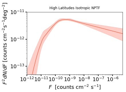
3. Plot Source Count Distributions

an.plot_source_count_median('iso_np',smin=0.01,smax=1000000,nsteps=10000,color='tomato',spow=2)
an.plot_source_count_band('iso_np',smin=0.01,smax=1000000,nsteps=10000,qs=[0.16,0.5,0.84],color='tomato',alpha=0.3,spow=2)

plt.yscale('log')
plt.xscale('log')
plt.xlim([1e-12,5e-6])
plt.ylim([5e-14,1e-11])
plt.tick_params(axis='x', length=5, width=2, labelsize=18)
plt.tick_params(axis='y', length=5, width=2, labelsize=18)
plt.ylabel('$F^2 dN/dF$ [counts cm$^{-2}$s$^{-1}$deg$^{-2}$]', fontsize=18)
plt.xlabel('$F$  [counts cm$^{-2}$ s$^{-1}$]', fontsize=18)
plt.title('High Latitudes Isotropic NPTF', y=1.02)

Text(0.5,1.02,'High Latitudes Isotropic NPTF')

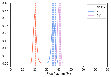
4. Plot Intensity Fractions

an.plot_intensity_fraction_non_poiss('iso_np', bins=100, color='tomato', label='Iso PS')
an.plot_intensity_fraction_poiss('iso', bins=100, color='cornflowerblue', label='Iso')
an.plot_intensity_fraction_poiss('dif', bins=100, color='plum', label='Dif')
plt.xlabel('Flux fraction (%)')
plt.legend(fancybox = True)
plt.xlim(0,80);

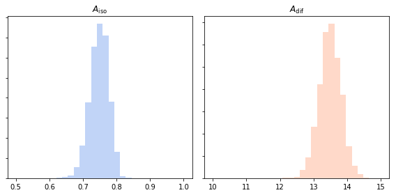
5. Access Parameter Posteriors

Poissonian parameters

Aiso_poiss_post = an.return_poiss_parameter_posteriors('iso')
Adif_poiss_post = an.return_poiss_parameter_posteriors('dif')

f, axarr = plt.subplots(1, 2);
f.set_figwidth(8)
f.set_figheight(4)


axarr[0].hist(Aiso_poiss_post, histtype='stepfilled', color='cornflowerblue', bins=np.linspace(.5,1,30),alpha=0.4);
axarr[0].set_title('$A_\mathrm{iso}$')
axarr[1].hist(Adif_poiss_post, histtype='stepfilled', color='lightsalmon', bins=np.linspace(10,15,30),alpha=0.4);
axarr[1].set_title('$A_\mathrm{dif}$')

plt.setp([a.get_yticklabels() for a in axarr[:]], visible=False);

plt.tight_layout()

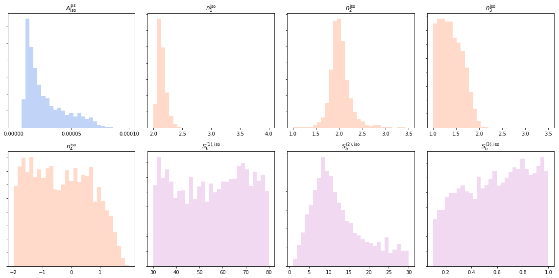
Non-poissonian parameters

Aiso_non_poiss_post, n_non_poiss_post, Sb_non_poiss_post = an.return_non_poiss_parameter_posteriors('iso_np')

f, axarr = plt.subplots(2, 4);
f.set_figwidth(16)
f.set_figheight(8)

axarr[0, 0].hist(Aiso_non_poiss_post, histtype='stepfilled', color='cornflowerblue', bins=np.linspace(0,.0001,30),alpha=0.4);
axarr[0, 0].set_title('$A_\mathrm{iso}^\mathrm{ps}$')
axarr[0, 1].hist(n_non_poiss_post[0], histtype='stepfilled', color='lightsalmon', bins=np.linspace(2,4,30),alpha=0.4);
axarr[0, 1].set_title('$n_1^\mathrm{iso}$')
axarr[0, 2].hist(n_non_poiss_post[1], histtype='stepfilled', color='lightsalmon', bins=np.linspace(1,3.5,30),alpha=0.4);
axarr[0, 2].set_title('$n_2^\mathrm{iso}$')
axarr[0, 3].hist(n_non_poiss_post[2], histtype='stepfilled', color='lightsalmon', bins=np.linspace(1,3.5,30),alpha=0.4);
axarr[0, 3].set_title('$n_3^\mathrm{iso}$')
axarr[1, 0].hist(n_non_poiss_post[3], histtype='stepfilled', color='lightsalmon', bins=np.linspace(-2,2,30),alpha=0.4);
axarr[1, 0].set_title('$n_4^\mathrm{iso}$')
axarr[1, 1].hist(Sb_non_poiss_post[0], histtype='stepfilled', color='plum', bins=np.linspace(30,80,30),alpha=0.4);
axarr[1, 1].set_title('$S_b^{(1), \mathrm{iso}}$')
axarr[1, 2].hist(Sb_non_poiss_post[1], histtype='stepfilled', color='plum', bins=np.linspace(1,30,30),alpha=0.4);
axarr[1, 2].set_title('$S_b^{(2), \mathrm{iso}}$')
axarr[1, 3].hist(Sb_non_poiss_post[2], histtype='stepfilled', color='plum', bins=np.linspace(0.1,1,30),alpha=0.4);
axarr[1, 3].set_title('$S_b^{(3), \mathrm{iso}}$')

plt.setp(axarr[0, 0], xticks=[x*.00005 for x in range(3)])
plt.setp(axarr[1, 0], xticks=[x*1.-2.0 for x in range(4)])
plt.setp(axarr[1, 3], xticks=[x*0.2+0.2 for x in range(5)])
plt.setp([a.get_yticklabels() for a in axarr[:, 0]], visible=False);
plt.setp([a.get_yticklabels() for a in axarr[:, 1]], visible=False);
plt.setp([a.get_yticklabels() for a in axarr[:, 2]], visible=False);
plt.setp([a.get_yticklabels() for a in axarr[:, 3]], visible=False);
plt.tight_layout()