Example 2: Creating Masks
In this example we show how to create masks using create_mask.py.
Often it is convenient to consider only a reduced Region of Interest
(ROI) when analyzing the data. In order to do this we need to create a
mask. The masks are boolean arrays where pixels labelled as True are
masked and those labelled False are unmasked. In this notebook we
give examples of how to create various masks.
The masks are created by create_mask.py and can be passed to an
instance of nptfit via the function load_mask for a run, or an
instance of dnds_analysis via load_mask_analysis for an
analysis. If no mask is specified the code defaults to the full sky as
the ROI.
NB: Before you can call functions from NPTFit, you must have it installed. Instructions to do so can be found here:
# Import relevant modules

%matplotlib inline
%load_ext autoreload
%autoreload 2

import numpy as np
import healpy as hp

from NPTFit import create_mask as cm # Module for creating masks
Example 1: Mask Nothing
If no options are specified, create mask returns an empty mask. In the plot here and for those below, purple represents unmasked, yellow masked.
example1 = cm.make_mask_total()
hp.mollview(example1, title='', cbar=False, min=0,max=1)

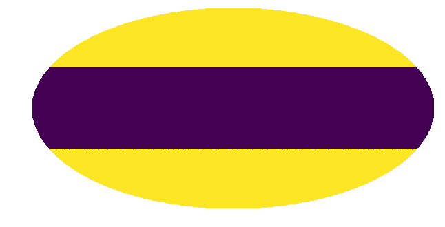
Example 2: Band Mask
Here we show an example of how to mask a region either side of the plane - specifically we mask 30 degrees either side
example2 = cm.make_mask_total(band_mask = True, band_mask_range = 30)
hp.mollview(example2, title='', cbar = False, min=0, max=1)

Example 3: Mask outside a band in b and l
This example shows several methods of masking outside specified regions in galactic longitude (l) and latitude (b). The third example shows how when two different masks are specified, the mask returned is the combination of both.
example3a = cm.make_mask_total(l_mask = False, l_deg_min = -30, l_deg_max = 30,
                               b_mask = True, b_deg_min = -30, b_deg_max = 30)
hp.mollview(example3a,title='',cbar=False,min=0,max=1)

example3b = cm.make_mask_total(l_mask = True, l_deg_min = -30, l_deg_max = 30,
                               b_mask = False, b_deg_min = -30, b_deg_max = 30)
hp.mollview(example3b,title='',cbar=False,min=0,max=1)

example3c = cm.make_mask_total(l_mask = True, l_deg_min = -30, l_deg_max = 30,
                              b_mask = True, b_deg_min = -30, b_deg_max = 30)
hp.mollview(example3c,title='',cbar=False,min=0,max=1)


Example 4: Ring and Annulus Mask
Next we show examples of masking outside a ring or annulus. The final example demonstrates that the ring need not be at the galactic center.
example4a = cm.make_mask_total(mask_ring = True, inner = 0, outer = 30, ring_b = 0, ring_l = 0)
hp.mollview(example4a,title='',cbar=False,min=0,max=1)

example4b = cm.make_mask_total(mask_ring = True, inner = 30, outer = 180, ring_b = 0, ring_l = 0)
hp.mollview(example4b,title='',cbar=False,min=0,max=1)

example4c = cm.make_mask_total(mask_ring = True, inner = 30, outer = 90, ring_b = 0, ring_l = 0)
hp.mollview(example4c,title='',cbar=False,min=0,max=1)

example4d = cm.make_mask_total(mask_ring = True, inner = 0, outer = 30, ring_b = 45, ring_l = 45)
hp.mollview(example4d,title='',cbar=False,min=0,max=1)


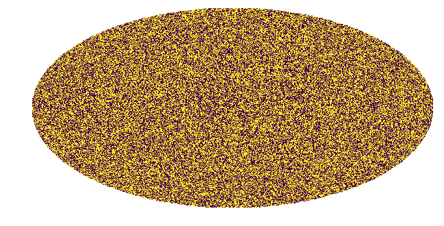
Example 5: Custom Mask
In addition to the options above, we can also add in custom masks. In this example we highlight this by adding a random mask.
random_custom_mask = np.random.choice(np.array([True, False]), hp.nside2npix(128))
example5 = cm.make_mask_total(custom_mask = random_custom_mask)
hp.mollview(example5,title='',cbar=False,min=0,max=1)
Example 6: Full Analysis Mask including Custom Point Source Catalog Mask
Finally we show an example of a full analysis mask that we will use for an analysis of the Galactic Center Excess in Example 3 and 8. Here we mask the plane with a band mask, mask outside a ring and also include a custom point source mask. The details of the point source mask are given in Example 1.
NB: before the point source mask can be loaded, the Fermi Data needs to be downloaded. See details in Example 1.
pscmask=np.array(np.load('fermi_data/fermidata_pscmask.npy'), dtype=bool)
example6 = cm.make_mask_total(band_mask = True, band_mask_range = 2,
                              mask_ring = True, inner = 0, outer = 30,
                              custom_mask = pscmask)
hp.mollview(example6,title='',cbar=False,min=0,max=1)