Example 10: Analyzing the Results of the High-Lat Run

In this Example we analyze the results of an MPI run of NPTFit performed over high latitudes.

The example batch script we provide, Example10_HighLat_Batch.batch is for SLURM. This calls the run file Example10_HighLat_Run.py using MPI, and is an example of how to perform a more realistic analysis using NPTFit.

NB: The batch file must be run before this notebook.

NB: This example makes use of the Fermi Data, which needs to already be installed. See Example 1 for details.

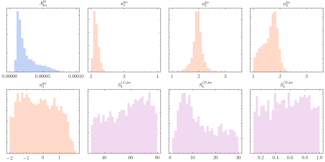
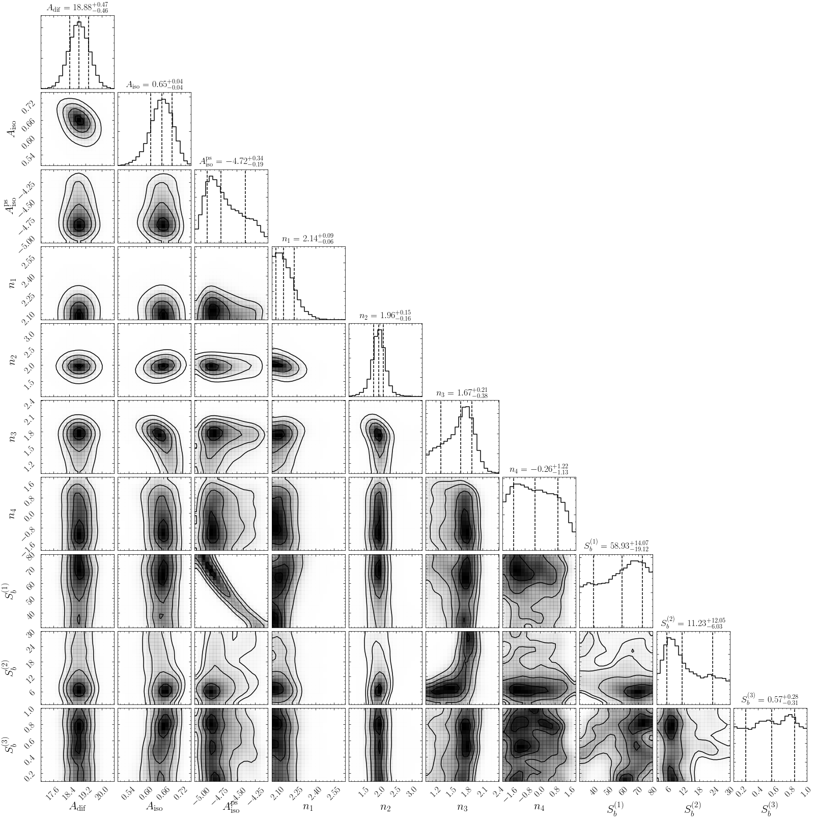
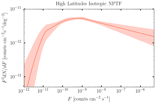
In this example, we model the source-count function as a triply-broken power law. In detail, the source count function is then:

\[\begin{split}\frac{dN}{dS} = A \left\{ \begin{array}{lc} \left( \frac{S}{S_{b,1}} \right)^{-n_1}, & S \geq S_{b,1} \\ \left(\frac{S}{S_{b,1}}\right)^{-n_2}, & S_{b,1} > S \geq S_{b,2} \\ \left( \frac{S_{b,2}}{S_{b,1}} \right)^{-n_2} \left(\frac{S}{S_{b,2}}\right)^{-n_3}, & S_{b,2} > S \geq S_{b,3} \\ \left( \frac{S_{b,2}}{S_{b,1}} \right)^{-n_2} \left( \frac{S_{b,3}}{S_{b,2}} \right)^{-n_3} \left(\frac{S}{S_{b,3}}\right)^{-n_4}, & S_{b,3} > S \end{array} \right.\end{split}\]

and is thereby described by the following eight parameters:

\[\theta = \left[ A, n_1, n_2, n_3, n_4, S_b^{(1)}, S_b^{(2)}, S_b^{(3)} \right]\,.\]

This provides an example of a more complicated source count function, and also explains why the run needs MPI.

Load in scan

We need to create an instance of nptfit.NPTF and load in the scan performed using MPI.

Loading the psf correction from: /group/hepheno/smsharma/NPTFit/examples/psf_dir/gauss_128_0.181_10_50000_1000_0.01.npy

The number of parameters to be fit is 10

Finally, load the completed scan performed using MPI.

analysing data from /group/hepheno/smsharma/NPTFit/examples/chains/HighLat_Example/.txt

Analysis

As in Example 9 we first initialize the analysis module. We will provide the same basic plots as in that notebook, where more details on each option is provided.

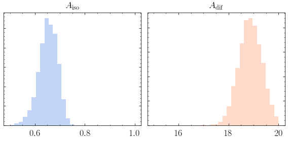
1. Make triangle plots

2. Get Intensities

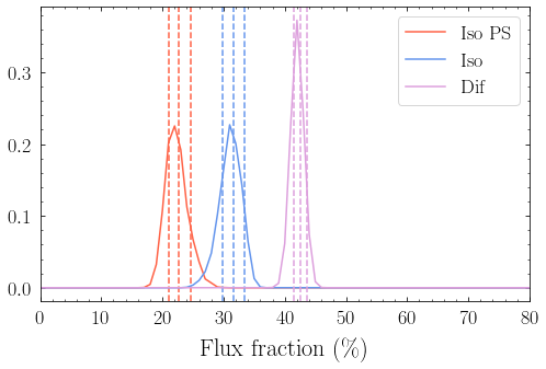
Iso NPT Intensity [  1.21483730e-07   1.31199062e-07   1.41996475e-07] ph/cm^2/s
Iso PT Intensity [  1.40131525e-07   1.48859129e-07   1.56973582e-07] ph/cm^2/s
Dif PT Intensity [  1.96440673e-07   2.01367819e-07   2.06396272e-07] ph/cm^2/s

3. Plot Source Count Distributions

<matplotlib.text.Text at 0x7f120cab7bd0>

4. Plot Intensity Fractions

5. Access Parameter Posteriors

Poissonian parameters

Non-poissonian parameters