Example 7: Manual evaluation of non-Poissonian Likelihood
In this example we show to manually evaluate the non-Poissonian
likelihood. This can be used, for example, to interface nptfit with
parameter estimation packages other than MultiNest. We also show how to
extract the prior cube.
We will take the exact same analysis as considered in the previous example, and show the likelihood peaks at exactly the same location for the normalisation of the non-Poissonian template.
NB: This example makes use of the Fermi Data, which needs to already be installed. See Example 1 for details.
Setup an identical instance of NPTFit to Example 6
Firstly we initialize an instance of nptfit identical to that used
in the previous example.
Loading the psf correction from: /zfs/nrodd/CodeDev/RerunNPTFExDiffFix/psf_dir/gauss_128_0.181_10_50000_1000_0.01.npy
The number of parameters to be fit is 3
Evaluate the Likelihood Manually
After configuring for the scan, the instance of nptfit.NPTF now has
an associated function ll. This function was passed to MultiNest in
the previous example, but we can also manually evaluate it.
The log likelihood function is called as: ll(theta), where theta
is a flattened array of parameters. In the case above:
As an example we can evaluate it at a few points around the best fit parameters:
Vary A:  -587.122352024368 -586.130196097067 -588.0937820199872
Vary n1: -586.1007629900672 -586.130196097067 -586.2930087056609
Vary n2: -587.2239543224257 -586.130196097067 -587.4195252590384
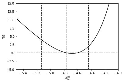
To make the point clearer we can fix \(n_1\) and \(n_2\) to their best fit values, and calculate a Test Statistics (TS) array as we vary \(\log_{10} \left( A^\mathrm{ps}_\mathrm{iso} \right)\). As shown the likelihood is maximised at approximated where MultiNest told us was the best fit point for this parameter.
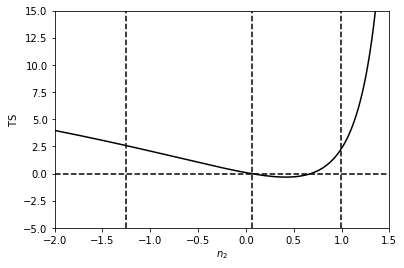
Next we do the same thing for \(n_2\). This time we see that this parameter is much more poorly constrained than the value of the normalisation, as the TS is very flat.
NB: it is important not to evaluate breaks exactly at a value of \(n=1\). The reason for this is the analytic form of the likelihood involves \((n-1)^{-1}\).
In general \(\theta\) will always be a flattened array of the
floated parameters. Poisson parameters always occur first, in the order
in which they were added (via add_poiss_model), following by
non-Poissonian parameters in the order they were added (via
add_non_poiss_model). To be explicit if we have \(m\) Poissonian
templates and \(n\) non-Poissonian templates with breaks
\(\ell_n\), then:
Fixed parameters are deleted from the list, and any parameter entered with a log flat prior is replaced by \(\log_{10}\) of itself.
Extract the Prior Cube Manually
To extract the prior cube, we use the internal function
log_prior_cube. This requires two arguments: 1. cube, the unit
cube of dimension equal to the number of floated parameters; and 2.
ndim, the number of floated parameters.
[1.0, 30.0, 1.9500000000000002]