Example 5: NPTF Correction for the Point Spread Function (PSF)

In this example we show how to account for the PSF correction using psf_correction.py

Fundamentally the presence of a non-zero PSF implies that the photons from any point source will be smeared out into some region around its true location. This effect must be accounted for in the NPTF. This is achieved via a function \(\rho(f)\). In the code we discretize \(\rho(f)\) as an approximation to the full function.

The two outputs of an instance of psf_correction are: 1. f_ary, an array of f values; and 2. df_rho_div_f_ary, an associated array of \(\Delta f \rho(f)/f\) values, where \(\Delta f\) is the width of the f_ary bins.

If the angular reconstruction of the data is perfect, then \(\rho(f) = \delta(f-1)\). In many situations, such as for the Fermi data at higher energies, a Gaussian approximation of the PSF will suffice. Even then there are a number of variables that go into evaluating the correction, as shown below. Finally we will show how the code can be used for the case of non-Gaussian PSFs.

As the calculation of \(\rho(f)\) can be time consuming, we always save the output to avoid recomputing the same correction twice. Consequently it can be convenient to have a common psf_dir where all PSF corrections for the runs are stored.

Example 1: Default Gaussian PSF

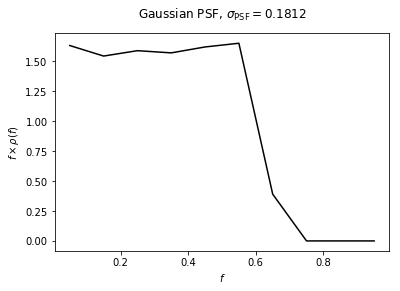
We start by showing the PSF correction for a Gaussian PSF - that is the PSF as a function of \(r\) is \(\exp \left[ -r^2 / (2\sigma^2) \right]\) - with \(\sigma\) set to the value of the 68% containment radius for the PSF of the Fermi dataset we will use in later examples.

File saved as: /zfs/nrodd/CodeDev/RerunNPTFExDiffFix/psf_dir/gauss_128_0.181_10_50000_1000_0.01.npy
f_ary: [0.05 0.15 0.25 0.35 0.45 0.55 0.65 0.75 0.85 0.95]
df_rho_div_f_ary: [65.29502702  6.86435887  2.543033    1.28251213  0.80024078  0.54595125
  0.09246876  0.          0.          0.        ]

Text(0.5,1.04,'Gaussian PSF, $\sigma_\mathrm{PSF} = 0.1812$')

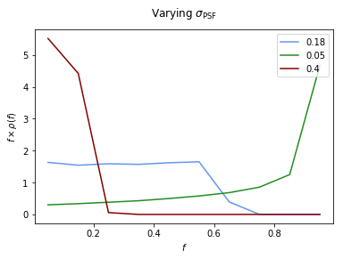
Example 2: Impact of changing \(\sigma\)

Here we show the impact on the PSF of changing \(\sigma\). From the plot we can see that for a small PSF, \(\rho(f)\) approaches the no PSF case of \(\delta(f-1)\) implying that the flux fractions are concentrated at a single large value. As \(\sigma\) increases we move away from this idealized scenario and the flux becomes more spread out, leading to a \(\rho(f)\) peaked at lower flux values.

File saved as: /zfs/nrodd/CodeDev/RerunNPTFExDiffFix/psf_dir/gauss_128_0.05_10_50000_1000_0.01.npy
File saved as: /zfs/nrodd/CodeDev/RerunNPTFExDiffFix/psf_dir/gauss_128_0.4_10_50000_1000_0.01.npy

Text(0.5,1.04,'Varying $\sigma_\mathrm{PSF}$')

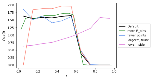
Example 3: Changing the default options for determining \(\rho(f)\)

In this example we show how for a given PSF, the other parameters associated with how accurately we calculate \(\rho(f)\) can impact what we get back. The parameters that can be changed are are:

Argument	Defaults	Purpose
num_f_bins	10	number of f_bins used
n_psf	50000	number of PSFs placed down when calculating
n_pts_per_psf	1000	number of points to place per psf in the calculation
f_trunc	0.01	minimum flux fraction to keep track of
nside	128	nside of the map the PSF is used on

The default parameters have been chosen to be accurate enough for the Fermi analyses we will be performed later. But if the user changes the PSF (even just \(\sigma\)), it is important to be sure that the above parameters are chosen so that \(\rho(f)\) is evaluated accurately enough.

In general increasing num_f_bins, n_psf, and n_pts_per_psf, whilst decreasing f_trunc leads to a more accurate \(\rho(f)\). But each will also slow down the evaluation of \(\rho(f)\), and in the case of num_f_bin, slow down the subsequent non-Poissonian likelihood evaluation.

nside should be set to the value of the map being analysed, but we also highlight the impact of changing it below. For an analysis on a non-HEALPix grid, the PSF can often be approximated by an appropriate HEALPix binning. If this is not the case, however, a different approach must be pursued in calculating \(\rho(f)\).

File saved as: /zfs/nrodd/CodeDev/RerunNPTFExDiffFix/psf_dir/gauss_128_0.181_20_50000_1000_0.01.npy
File saved as: /zfs/nrodd/CodeDev/RerunNPTFExDiffFix/psf_dir/gauss_128_0.181_10_5000_100_0.01.npy
File saved as: /zfs/nrodd/CodeDev/RerunNPTFExDiffFix/psf_dir/gauss_128_0.181_10_50000_1000_0.1.npy
File saved as: /zfs/nrodd/CodeDev/RerunNPTFExDiffFix/psf_dir/gauss_64_0.181_10_50000_1000_0.01.npy

<matplotlib.legend.Legend at 0x7f393e0dc470>

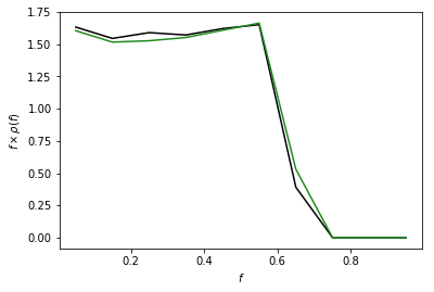
Example 4: PSF on a Cartesian Grid

For some applications, particularly when analyzing smaller regions of the sky, it may be desirable to work with data on a Cartesian grid rather than a healpix map. Note generally for larger regions, in order to account for curvature on the sky a healpix pixelization is recommended. Code to convert from Cartesian grids to healpix can be found here: https://github.com/nickrodd/grid2healpix

In order to calculate the appropriate PSF correction for Cartesian maps the general syntax is the same, except now the healpix_map keyword should be set to False and the pixarea keyword set to the area in sr of each pixel of the Cartesian map. In addition the gridsize keyword determines how large the map is, and flux that falls outside the map is lost in the Cartesian case.

As an example of this syntax we calculate the PSF correction on a Cartesian map that has pixels the same size as an nside=128 healpix map, and compare the two PSF corrections. Note they are essentially identical.

File saved as: /zfs/nrodd/CodeDev/RerunNPTFExDiffFix/psf_dir/gauss_0.21_0.181_10_50000_1000_0.01.npy

Text(0,0.5,'$f \times \rho(f)$')

Example 5: Custom PSF

In addition to the default Gausian PSF, psf_correction.py also has the option of taking in a custom PSF. In order to use this ability, the user needs to initialise psf_correction with delay_compute=True, manually define the parameters that define the PSF and then call make_or_load_psf_corr.

The variables that need to be redefined in the instance of psf_correction are:

Argument	Purpose
psf_r_func	the psf as a function of r, distance in radians from the center of the point source
sample_psf_m ax	maximum distance to sample the psf from the center, should be larger for psfs with long tails
``psf_samples` `	number of samples to make from the psf (linearly spaced) from 0 to sample_psf_m ax, should be large enough to adequately represent the full psf
psf_tag	label the psf is saved with

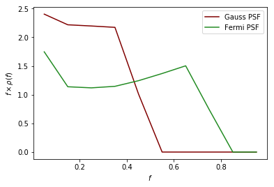
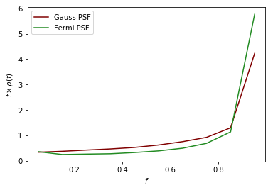
As an example of a more complicated PSF we consider the full Fermi-LAT PSF. The PSF of Fermi is approximately Gaussian near the core, but has larger tails. To model this a pair of King functions are used to describe the radial distribution. Below we show a comparison between the Gaussian approximation and the full PSF, for two different energies. As shown, for low energies where the Fermi PSF is larger, the difference between the two can be significant. For higher energies where the PSF becomes smaller, however, the difference is marginal.

For the full details of the Fermi-LAT PSF, see: http://fermi.gsfc.nasa.gov/ssc/data/analysis/documentation/Cicerone/Cicerone_LAT_IRFs/IRF_PSF.html

File saved as: /zfs/nrodd/CodeDev/RerunNPTFExDiffFix/psf_dir/gauss_128_0.235_10_50000_1000_0.01.npy
File saved as: /zfs/nrodd/CodeDev/RerunNPTFExDiffFix/psf_dir/Fermi_PSF_2GeV.npy

<matplotlib.legend.Legend at 0x7f393e00dd30>

File saved as: /zfs/nrodd/CodeDev/RerunNPTFExDiffFix/psf_dir/gauss_128_0.055_10_50000_1000_0.01.npy
File saved as: /zfs/nrodd/CodeDev/RerunNPTFExDiffFix/psf_dir/Fermi_PSF_20GeV.npy

<matplotlib.legend.Legend at 0x7f393df7a8d0>

The above example also serves as a tutorial on how to combine various PSFs into a single PSF. In the case of the Fermi PSF the full radial dependence is the sum of two King functions. More generally if the full PSF is a combination of multiple individual ones (for example from multiple energy bins), then this can be formed by just adding these functions with an appropriate weighting to get a single psf_r_func.